GenePlexus Help Page
The help page provides various help, advice, and interpretation of the various inputs and outputs on the GenePlexus webserver.
Inputs
- Supplying input genes
- Choosing a molecular network
- Choosing a way to represent network features
- Choosing negative genes
- Guidelines for choosing the best job settings
- Effect of the user-supplied gene set on model performance
Supplying input genes
The user can supply a list of genes by either uploading a file of genes or manually entering the genes in a text box. In both cases, each gene needs to be on a new line.
Here is an example gene list file : download DOID-9562-STRING-Adjacency-DisGeNet-Symbols.txt
The following types of gene IDs are allowed as inputs:
- Entrez
- Symbol
- ENSG (Ensembl gene)
- ENSP (Ensembl protein)
- ENST (Ensembl transcript)
Note: The Ensembl IDs (ENSG, ESNP, ENST) cannot contain any version numbers.
The genes supplied by the user will be converted to Entrez gene identifiers using gene ID mappings obtained from 60,000 locally downloaded human gene files from mygene.info.
After uploading/entering the genes, users can validate their input list by clicking the Validate button. This will pop up two tables:
- A table that shows the original gene IDs the user supplied and their corresponding Entrez gene IDs. The last four columns indicate whether or not the gene is present in each of the networks in GenePlexus.
- A table that shows for each network, the total number of genes in that network and how many among them are also part of the user supplied gene list.
Choosing a molecular network
The user can choose between four human genome-scale molecular networks. For each network, the nodes are mapped into Entrez gene IDs. For the GIANT-TN network, the original network was additionally filtered to remove edges with scores below the prior probability (0.01).
- BioGRID (19,022 genes, 484,356 edges). This network is a relatively sparse unweighted network with high gene coverage. The edges in the network are only from verified experimental results.
- STRING (18,582 genes, 5,521,113 edges). This network is a moderately well-connected weighted network that integrates information from multiple sources (experimental results, homology, annotation databases, etc).
- STRING-EXP (17,417 genes, 2,121,428 edges). This network contains only the "experimental" edges from the STRING network.
- GIANT-TN (25,689 genes, 38,904,929 edges). This is a nearly fully-connected weighted network that is derived from combining data from co-expression networks generated across 1000s of gene expression experiments along with gene interaction information from a few other sources including protein interactions. In this webserver, we use the tissue-naive GIANT network.
Choosing a way to represent network features
When a network is to be used in a supervised machine learning model, the network connections can be represented as features in one of three ways:
- Adjacency. This method uses the network edges directly from the molecular networks. This feature type might work best for the
STRINGandSTRING-EXPnetworks. - Influence. The edge information in the original network is diffused over all edges using a random walk with restart technique. This feature type works best for dense networks where many edges may be a bit “noisy”, so here it might be best to use with
GIANT-TN. - Embedding. The connectivity of a given gene in the network to all the other genes is represented with a low dimensional numerical vector using the node2vec algorithm. This feature type works best with sparse networks, so here it might be best to use with
BioGRID.
Choosing negative genes
In the supervised machine learning model, any gene from the user-supplied gene list that is able to be converted to an Entrez ID and is also in the network is considered part of the positive class. The user can then choose if they want to define genes in the negative class based on one of two geneset collections, Gene Ontology Biological Processes or DisGeNet, based on whether the input genes represent a cellular process/pathway or a disease.
GenePlexus then automatically selects the genes in the negative class by:
- Retaining all terms in the selected geneset collection that have between 10 and 200 genes annotated to them.
- Considering the total pool of possible negative genes to be any gene that has an annotation to at least one of the terms in the selected geneset collection.
- Removing genes that are in the positive class.
- Performing a hypergeometric test between the genes in the positive class and the lists of genes annotated to every term in the selected geneset collection. If the value of this hypergeometric test is less than 0.05, all genes from the given term are also removed from the pool of possible negative genes.
- Declaring all the remaining genes in the pool of possible negative genes as the negative class.
Guidelines for choosing the best job settings
The first step is choosing the network. If your gene set of interest comes from a curated database or it was generated while studying a specific process/pathway or disease, the best network to choose is STRING as this network is a highly curated network that uses prior knowledge from gene set databases in building the network. If you would like to only consider experimental interactions, then the network to use is STRING-EXP, and if you would further only like to consider physical interactions, choose BioGRID. The GIANT-TN network is best to use for two cases. First, since it offers the highest gene coverage, it enables the user to see predictions on many more understudied genes. Second, as GIANT-TN is a very dense network that does not directly incorporate gene set database information, this network performs well on larger gene sets that may be derived from high-throughput experiments.
The next step is to choose the way the network is represented as features in the machine learning model.
- For BioGIRD, using Adjacency or Embedding usually results very similar performance
- For STRING-EXP, using Adjacency is usually the best feature representation.
- For GIANT-TN, Influence is usually the best representation.
- For STRING, if your input gene set size is smaller or if the gene set is similar to a specific biological process, then using Adjacency is the best choice. If the gene set size is larger or if the gene set corresponds to a complex phenotype, then use Influence.
The next step is to choose the background used to determine the genes used as negative examples in the machine learning model. If your gene set corresponds to a biological process or pathway, choose GO. Instead, if it corresponds more closely to a disease or a complex phenotype, then choose DisGeNet.
The best way to determine if the chosen job options worked well is to look at the cross-validation score at the top of the results page. It could be useful to compare the cross validation score for a few different combinations of job options to help the user find the optimal set of options. Additionally, the figure below shows a summary of results generated from our recent work benchmarking GenePlexus and could help a user pick the best job parameters.
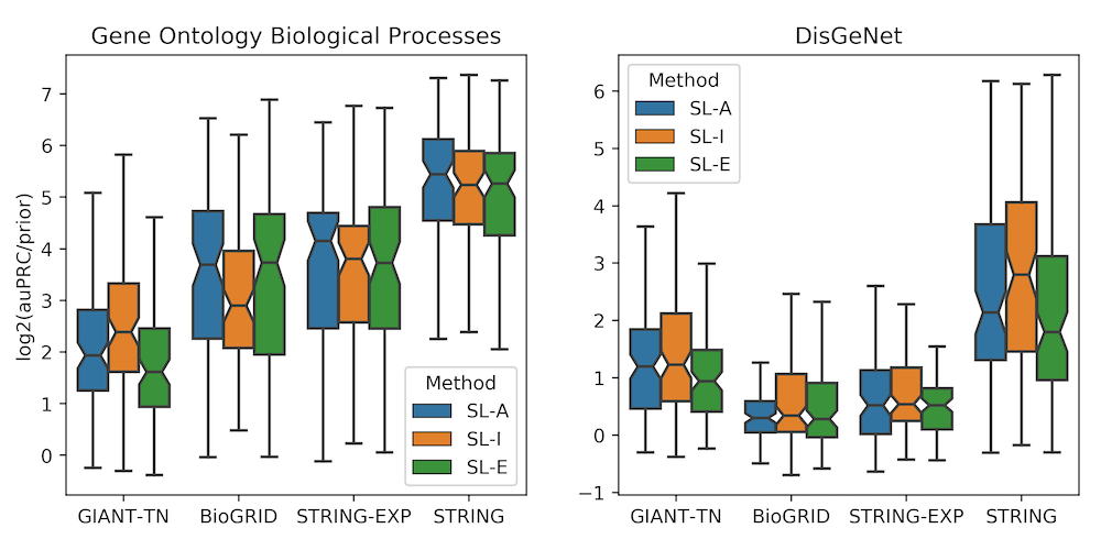
This figure displays results from the paper Supervised learning is an accurate method for network-based gene classification where the parameters are options in the GenePlexus webserver. The left panel is for models trained for Gene Ontology biological prcoesses and the right panel is for models trained for DisGeNet diseases. Each boxplot contains the results of anywhere between 89 and 160 models. Each model was trained using the study-bias holdout method, where for each geneset in a geneset collection, the most well studied genes were used to train the model and the least studied genes were used for testing. This figure can be used to help users pick the network, feature type and negative selection class that best suits their input gene list. It is worth noting that the STRING network is built in part by using Gene Ontology and DisGeNet annotations, and this circularity could be the reason for the enhanced performance of the STRING network in this evaluation.
Effect of the user-supplied gene set on model performance
The GenePlexus method has been extensively benchmarked on models that used between 10 and ~400 genes in the training set. We have found that, while there is some decrease in performance as the number of genes in the gene set increases (far left panel in the figure below), the major driving force is how “connected” the genes are in the network (center and right panel in the figure below). This is understandable as GenePlexus heavily leverages the underlying network when training the model. We have found that the GIANT-TN network shows the least decrease in performance as the gene set size increases and thus we recommend this network for use with larger gene sets like those that are generated directly from high-throughput experiments. As mentioned above, the cross-validation score is very useful in determining if a given model worked well on the user-supplied gene list.
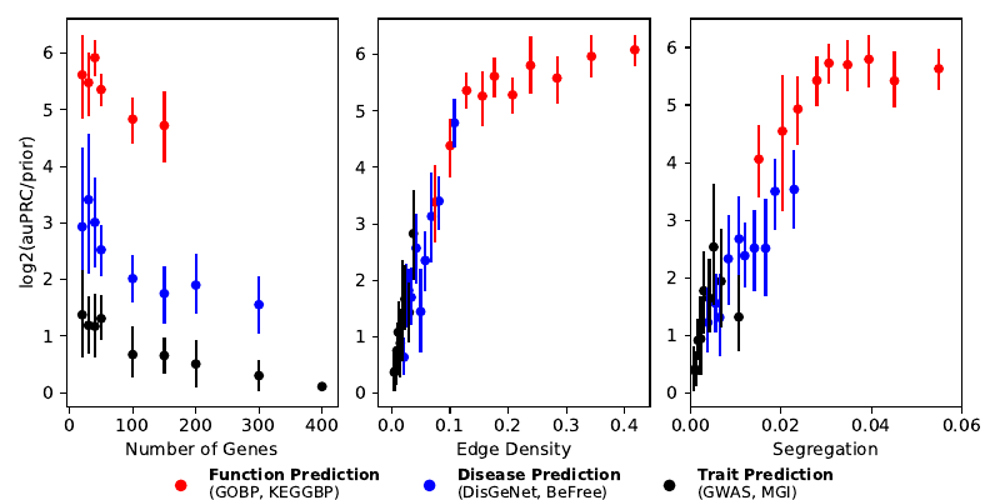
This figure shows results from the paper Supervised learning is an accurate method for network-based gene classification is an accurate method that looks into how different properties of the gene set affect the model performance. Here, the edge density is a measure of how connected a gene set is to itself in the network and segregation is how isolated the gene set is from the rest of the network. While there is decrease in performance as the number of genes is increased, the major driving force for the model is how connected the gene set is in the network. The results here are shown for the STRING network.
Outputs
- Information at the top
- Gene predictions
- Comparison to other pre-trained models
- Network graph
- Validation data
Information at the top
The box at the top displays the parameters of the job along with the job name. If the number of genes in the positive class is greater than 15, then the
results of 3-fold cross validation performance is displayed in terms of log2(auPRC/prior). This metric reports the 2-fold change of the area under the precision-recall curve (auPRC) over the prior auPRC expected by random chance. For example, a value of 1 indicates a model that performs twice as good as the expected result.
Gene predictions
This table contains the prediction probability for every gene in the network, indicating its membership in the positive class. The probabilities are bounded from 0 to 1 with 1 being the highest probability of being in the positive class.
The possible Known/Novel column values are:
- Known: These are genes that are in the positive class (supplied by the user).
- Novel: These are genes that are the predicted novel associations. These genes could have been part of the negative class or not used in training the model at all.
The possible Training-labels column values are:
- P: Gene was part of the positive class during training.
- N: Gene was part of the negative class during training.
- U: Gene was unused during training.
The table can be filtered by using the text box above the table. For example, often the top predictions are from genes in the positive class. So, it might be useful to type “Novel” into the text box to see what are the top predicted novel genes.
Clicking the Entrez Gene ID takes the user to a webpage containing more information on that gene.
Comparison to other pre-trained models
The tables here show how similar the custom model trained on the user-supplied gene list compares to other pre-trained models. The webserver stores the model weights from machine-learning models trained using lists of genes annotated to numerous Gene Ontology biological processes and DisGeNet diseases. The similarity score is determined by:
- Finding the cosine similarity between the model trained with the user-supplied gene list and all the model weights from the genesets in a geneset collection, where the model was trained using the same molecular network and feature type selected by the user.
- Reading in a pre-saved matrix containing the similarities between models from genesets in the geneset collection that was chosen to make the negative class and models for genesets in the geneset collection being displayed in the table.
- Adding the vector of similarities found in step one as a row in this matrix.
- Finding both the columnwise and rowwise z-scores for each element in this appended row where the columnwise z-score corrects for the background among terms using that negative set of genes and the rowwise z-score corrects for the background among all genesets displayed in the table.
- Calcualting the final similarity as the combination of these two z-scores combined using the l2-norm.
Clicking the Term ID takes the user to a page containing more information about that term.
Network graph
The top predictions from the supervised machine learning model are displayed, showing how they are connected to each other in the network used to train the machine learning model.
- The nodes are colored by which class they were in, with green indicating genes in the positive class, blue indicating genes not used in training, and red indicating genes in the negative class.
- The size of the nodes scales with the prediction probability, with the larger nodes having the higher prediction probability.
Validation data
The table here shows how the user input gene list was converted to Entrez IDs and if the converted Entrez IDs were in the network that was used to train the model.
Other Information
References
Web Server
Mancuso CA, Bills PS, Krum D, Newsted J, Liu R, Krishnan A. (2022) GenePlexus: a web-server for gene discovery using network-based machine learning, Nucleic Acids Research, gkac335 doi:10.1093/nar/gkac335.
Networks
GIANT
Greene CS, Krishnan A, Wong AK, Ricciotti E, Zelaya RA, Himmelstein DS, Zhang R, Hartmann BM, Zaslavsky E, Sealfon SC, Chasman DI, FitzGerald GA, Dolinski K, Grosser T, Troyanskaya OG. (2015) Understanding multicellular function and disease with human tissue-specific networks. Nature Genetics 47:569-576.
STRING and STRING-EXP
Szklarczyk,D., Gable,A.L., Lyon,D., Junge,A., Wyder,S., Huerta-Cepas,J., Simonovic,M., Doncheva,N.T., Morris,J.H., Bork,P., et al. (2019) STRING v11: protein–protein association networks with increased coverage, supporting functional discovery in genome-wide experimental datasets. Nucleic Acids Research, Nucleic Acids Research 47:D607–D613.
BioGRID
Stark C, Breitkreutz BJ, Reguly T, Boucher L, Breitkreutz A, Tyers M. (2006) BioGRID: a general repository for interaction datasets. Nucleic Acids Research 34:D535-539.
Oughtred,R., Stark,C., Breitkreutz,B.-J., Rust,J., Boucher,L., Chang,C., Kolas,N., O’Donnell,L., Leung,G., McAdam,R., et al. (2019) The BioGRID interaction database: 2019 update. Nucleic Acids Research, 47:D529–D541
Geneset collections
Gene Ontology
- Ashburner M, Ball CA, Blake JA, Botstein D, Butler H, Cherry JM, Davis AP, Dolinski K, Dwight SS, Eppig JT, Harris MA, Hill DP, Issel-Tarver L, Kasarskis A, Lewis S, Matese JC, Richardson JE, Ringwald M, Rubin GM, Sherlock G. (2000) Gene ontology: tool for the unification of biology. The Gene Ontology Consortium. Nature Genetics 25:25-29.
- The Gene Ontology Consortium. (2019) The Gene Ontology Resource: 20 years and still GOing strong. Nucleic Acids Research 47:D330-338.
DisGeNet
- Piñero J, Queralt-Rosinach N, Bravo À, Deu-Pons J, Bauer-Mehren A, Baron M, Sanz F, Furlong LI. (2015) DisGeNET: a discovery platform for the dynamical exploration of human diseases and their genes. Database bav028.
- Piñero J, Bravo À, Queralt-Rosinach N, Gutiérrez-Sacristán A, Deu-Pons J, Centeno E, García-García J, Sanz F, Furlong LI. (2017) DisGeNET: a comprehensive platform integrating information on human disease-associated genes and variants. Nucleic Acids Research 45:D833-839.
- Schriml LM, Mitraka E, Munro J, Tauber B, Schor M, Nickle L, Felix V, Jeng L, Bearer C, Lichenstein R, Bisordi K, Campion N, Hyman B, Kurland D, Oates CP, Kibbey S, Sreekumar P, Le C, Giglio M, Greene C. (2019) Human Disease Ontology 2018 update: classification, content and workflow expansion. Nucleic Acids Research 47:D955-D962.
Mygene.info
- Wu C, MacLeod I, Su AI (2013) BioGPS and MyGene.info: organizing online, gene-centric information. Nucleic Acids Research 41:D561-D565.
- Xin J, Mark A, Afrasiabi C, Tsueng G, Juchler M, Gopal N, Stupp GS, Putman TE, Ainscough BJ, Griffith OL, Torkamani A, Whetzel PL, Mungall CJ, Mooney SD, Su AI, Wu C (2016) High-performance web services for querying gene and variant annotation. Genome Biology 17:1-7.
License
The results of the GenePlexus webserver are licensed under the Creative Commons License: Attribution 4.0 International
License information for networks and genesets collections used in this work
- STRING, STRING-EXP and GO use the Creative Commons License: Attribution 4.0 International.
- DisGenet uses the Creative Commons License: Attribution-NonCommercial-ShareAlike 4.0 International.
- BioGRID and MyGene.info have terms of use on their websites (see below).
The location of the license agreement or terms-of-use for each network or geneset collection can be found by clicking the following links. We note that no license agreement was available for GIANT, however we have obtained permission from the owner of the material to redistribute the network and they have noted that they will be adding a Creative Commons License: Attribution-NonCommercial 4.0 International to the website soon.